Auto-Correlation Function Plots
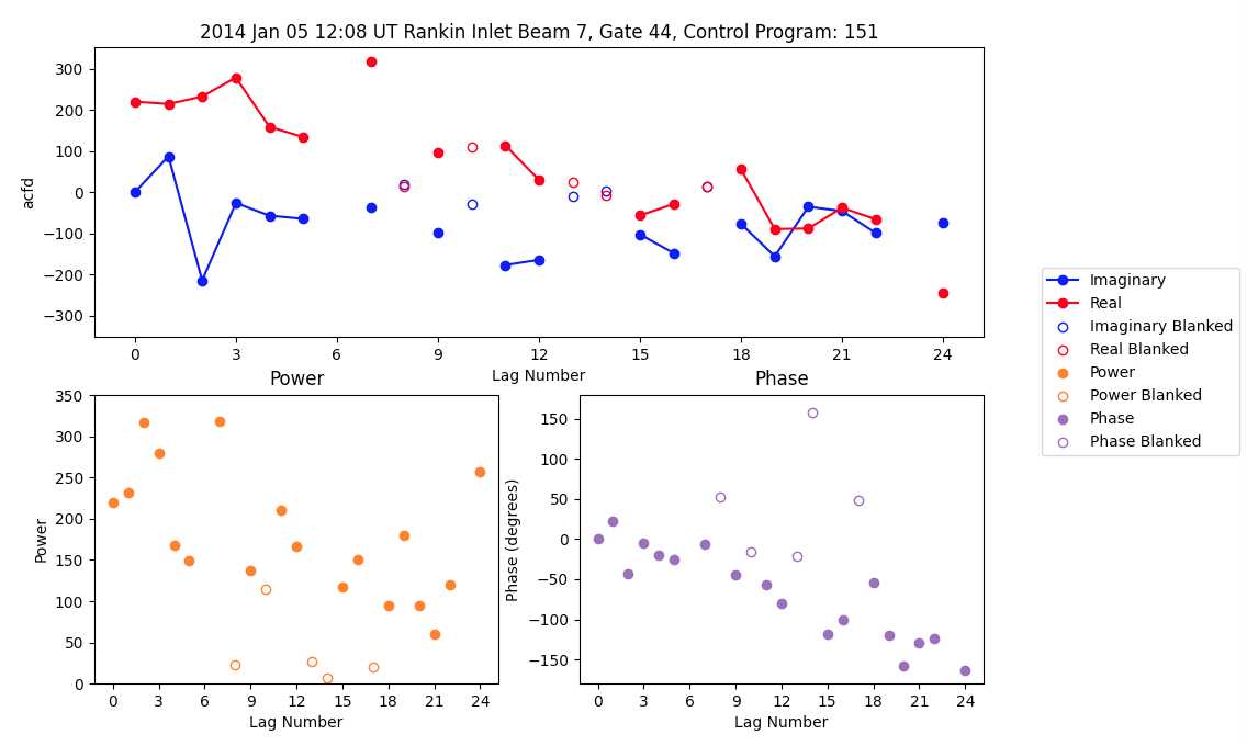
plot_acfs plots the imaginary and real parts of the Auto-Correlation Function (ACF), along with the power and phase of the ACF in the selected RAWACF file for a given range gate and beam.
Basic code to plot ACFs from a RAWACF file would look like:
import pydarn
import matplotlib.pyplot as plt
from datetime import datetime

rawacf_data, _ = pydarn.read_rawacf("data/20140105.1208.03.rkn.rawacf")
plt.figure(figsize=(12, 7))
pydarn.ACF.plot_acfs(rawacf_data, beam_num=7, gate_num=44,
                     start_time=datetime(2014, 1, 5, 12, 8))
plt.show()
You also have access to numerous plotting options:
| Parameter | Action |
|---|---|
| beam_num=(int) | Beam number to plot (default:0) |
| gate_num=(int) | Gate number to plot (default:15) |
| parameter=(string) | Parameter to pick between acfd or xcfd plotting (default: acdf) |
| scan_num=(int) | The scan number to plot (default:0) |
| start_time=None | Plot the closest beam scan to the given start time (overrides the scan number if set) |
| normalized=(bool) | Normalizes the parameter data with the associated power 0 value |
| real_color=(str) | Line color for real data |
| imaginary_color=(str) | Line color for imaginary data |
| plot_blank=(bool) | Determine if blanked lags should be plotted |
| blank_marker=(str) | Choice of marker to indicate blanked lags are a dot (general python markers accepted) |
| legend=(bool) | Plot a legend |
| pwr_and_phs=(bool) | Plots subplots of power and phase of the ACF |
| pwr_color=(str) | Line color for power data |
| phs_color=(str) | Line color for phase data |
| real_marker=(str) | Choice of marker for real data (general python markers accepted) |
| imaginary_marker=(str) | Choice of marker for imaginary data (general python markers accepted) |
| pwr_marker=(str) | Choice of marker for power data (general python markers accepted) |
| phs_marker=(str) | Choice of marker for phase data (general python markers accepted) |
| kwargs** | Arguments to pass in to matplotlib plot |
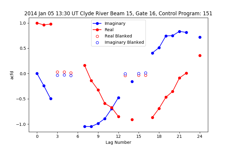
Another example that does not plot the power or phase and contains blanked lags is:
import pydarn
import matplotlib.pyplot as plt
from datetime import datetime

rawacf_file = 'data/20140105.1200.03.cly.rawacf'
rawacf_data, _ = pydarn.read_rawacf(rawacf_file)
pydarn.ACF.plot_acfs(rawacf_data, beam_num=15, gate_num=16,
                     start_time=datetime(2014, 1, 5, 13, 30),
                     pwr_and_phs=False)
plt.show()