Basic Time Series Plots

plot_time_series simply plots out a time series of any scalar beam parameter in FITACF or RAWACF files. See Map tutorial for map file scalar parameter plotting.

Basic code to plot a time series from a FITACF file would look like:

import matplotlib.pyplot as plt
import pydarn

file = "20190831.C0.cly.fitacf"
fitacf_data, _ = pydarn.read_fitacf(file)

pydarn.RTP.plot_time_series(fitacf_data)
plt.show()

If no scalar parameter is specified (using parameter=string), or beam (using beam_num=int), then the default is a tfreq time series from beam 0.

In a similar way to RTP, you also have access to numerous plotting options:

Parameter	Action
start_time=(datetime object)	Control the start time of the plot
end_time=(datetime object)	Control the end time of the plot
date_fmt=(string)	How the x-tick labels look. Default is ('%y/%m/%d\n %H:%M')
channel=(int or string)	Choose which channel to plot. Default is 'all'.
cp_name=(bool)	Print the name of the cpid when plotting cpid timeseries'
color=(str)	Color of the line plot
linestyle=(str)	Style of line plotted
linewidth=(float)	Thickness of plotted line

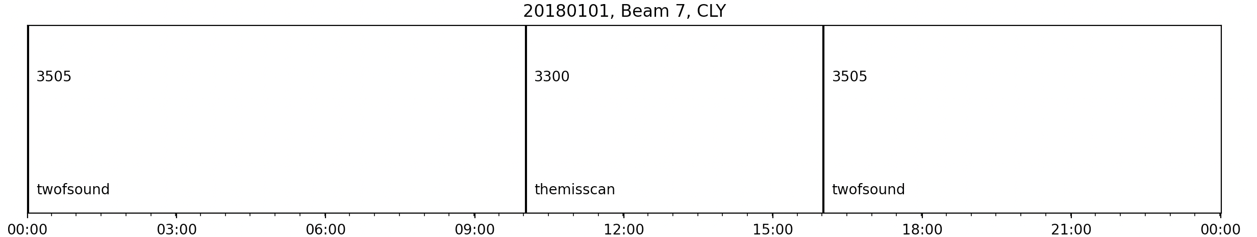
For example, this plot shows the cpids in a 24hour Clyde FITACF file:

plt.title("20180101, Beam 7, CLY")
pydarn.RTP.plot_time_series(fitacf_data, parameter='cp', date_fmt=('%H:%M'), beam_no=7)
plt.show()

Advanced Time Series Plots

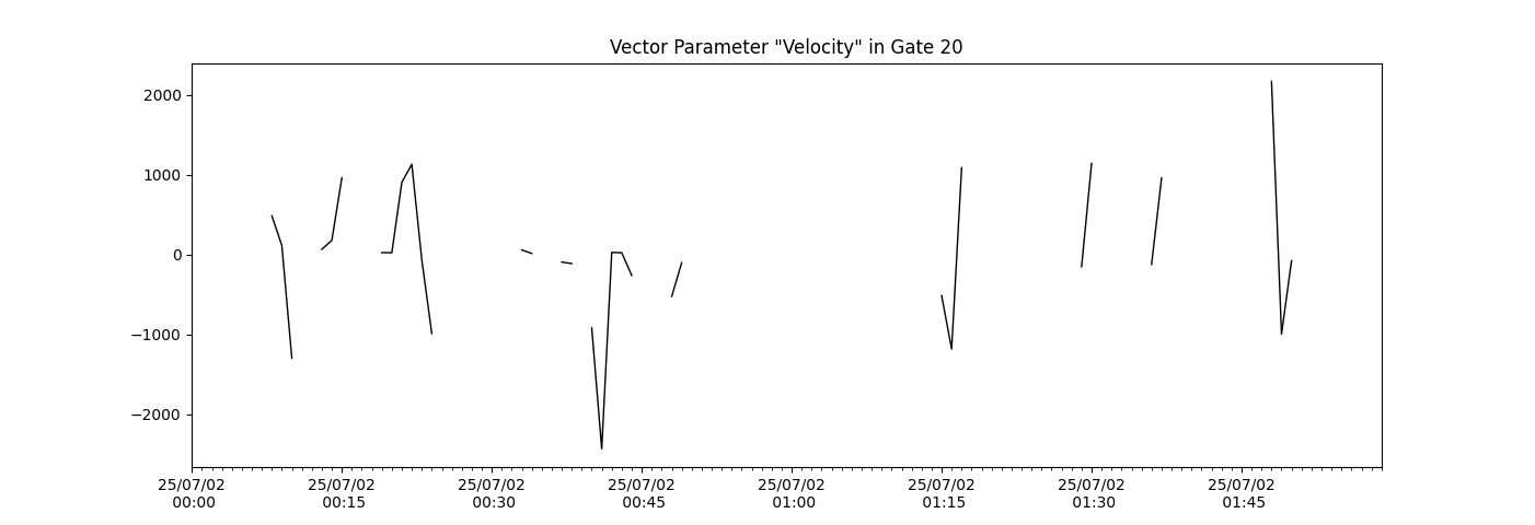
This method is flexible and can be used to plot any value as a time series. By choosing any parameter that matches a field name in any of the DMap files, you can plot that parameter as a time series. The user can also can choose a vector parameter, and then choose the gate in which you would like to plot the data with time using the gate option (e.g. gate=25).

fitacf_data,_ = pydarn.read_fitacf('20250702.0000.00.sas.a.fitacf')
plt.title('Vector Parameter "Velocity" in Gate 20')
pydarn.RTP.plot_time_series(fitacf_data, parameter='v', beam_no=7, gate=20)
plt.show()