Fan plots

---

Fan plots are a way to visualise data from the entire scan of a SuperDARN radar.

All beams and ranges for a given parameter (such as line-of-sight velocity, backscatter power, etc) and a particular scan can be projected onto a polar or geomagnetic plot in AACGMv2 coordinates, or projected onto a geographic plot in geographic coordinates.

Basic usage

import matplotlib.pyplot as plt
from datetime import datetime
import pydarn

file = "path/to/fitacf/file"
fitacf_data, _ = pydarn.read_fitacf(file)

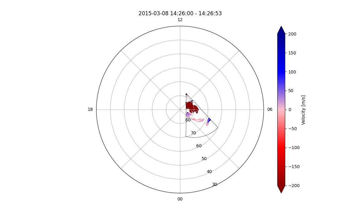
With the FITACF data loaded as a list of dictionaries (fitacf_data variable in above example), you may now call the plot_fan method. Make sure you tell it which scan (numbered from first recorded scan in file, counting from 1 or give it a datetime object for the scan at that time) you want using scan_index:

fan_rtn = pydarn.Fan.plot_fan(fitacf_data, scan_index=27, 
                              colorbar_label='Velocity [m/s]')
plt.show()

In this example, the 27th scan was plotted with the defaulted parameter being line-of-sight velocity:

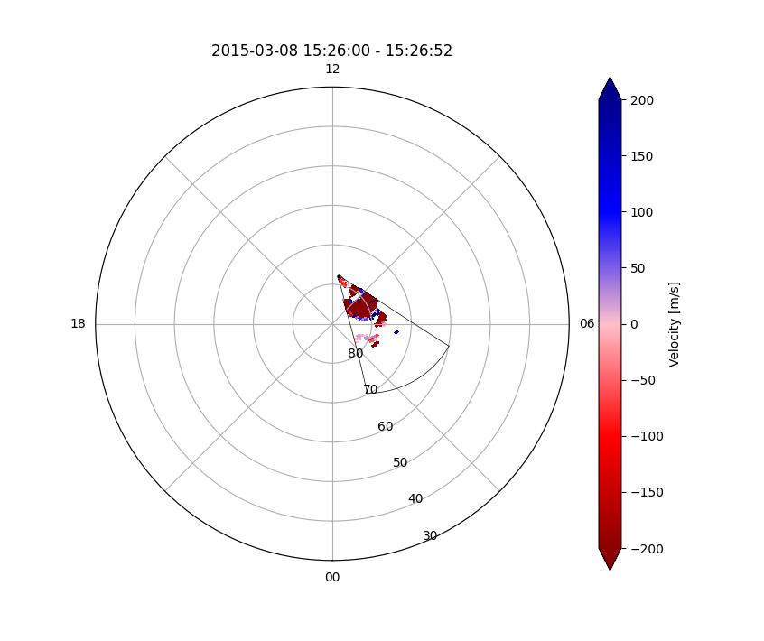
You can also provide a datetime object to obtain a scan at a specific time using the scan_time key word:

pydarn.Fan.plot_fan(fitacf_data, scan_time=datetime(2015, 3, 8, 15, 26),
                     colorbar_label='Velocity [m/s]')
plt.show()

Tolerance

You can also set a tolerance time as a timedelta object to plot only data a specific number of seconds around a datetime given. This is helpful to plot non-traditional scans and newer fast scans with a larger amount of data to separate.

If using scan_time, the user can also specify scan_time_tolerance as a datetime.timedelta object. The example code below will plot any data that is +/- 20 seconds around the time 2020-01-01 00:05:00 on a fan plot.

rtn = pydarn.Fan.plot_fan(fitacf_data,
                          scan_time=dt.datetime(2020,1,1,0,5),
                          scan_time_tolerance=dt.timedelta(seconds=20))
plt.show()

Groundscatter

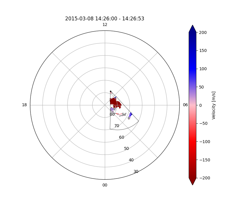
Default plots do not show groundscatter as grey. Set it to true to grey out groundscatter:

fan_rtn = pydarn.Fan.plot_fan(fitacf_data,
                              scan_index=27,
                              groundscatter=True)
plt.show()

Parameters Available for Plotting

In addition to line-of-sight velocity, you can choose one of three other data products to plot by setting parameter=String name:

Data product	String name
Line of sight velocity (m/s) [Default]	'v'
Spectral width (m/s)	'w_l'
Elevation angle (degrees)	'elv'
Power (dB)	'p_l'

Ball and Stick Plots

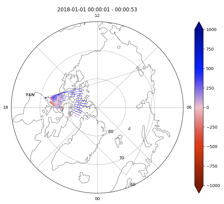
Data on fan plots can also be displayed as a 'ball and stick' plot, where each data point is represented by a ball with a stick showing direction towards or away from the radar, coloured by the magnitude of the parameter plotted. Ball and stick plots can be plotted usng the ball_and_stick with len_factor key words to control the size of the sticks, as follows:

pydarn.Fan.plot_fan(fitacf_data,
                    scan_index=1, lowlat=60, zmin=-1000, zmax=1000,
                    boundary=True, radar_label=True,
                    groundscatter=True, ball_and_stick=True, len_factor=300,
                    coastline=True, parameter="v")
plt.show()

Additional Options

Here is a list of all the current options than can be used with plot_fan

Option	Action
ax=(Axes Object)	Matplotlib axes object than can be used for cartopy additions
scan_index=(int)	Scan number, from start of records in file corresponding to channel if given
scan_time=(datetime)	Time of the scan required to plot (default uses scan_index=1)
scan_time_tolerance_=(timedelta)	Time difference around scan where data will need to be plotted (default 30 seconds)
channel=(int or 'all')	Specify channel number or choose 'all' (default = 'all')
parameter=(string)	See above table for options
groundscatter=(bool)	True or false to showing ground scatter as grey
ranges=(list)	Two element list giving the lower and upper ranges to plot, grabs ranges from hardware file (default []
cmap=string	A matplotlib color map string
grid=(bool)	Boolean to apply the grid lay of the FOV (default: False )
zmin=(int)	Minimum data value for colouring
zmax=(int)	Maximum data value for colouring
colorbar=(bool)	Set true to plot a colorbar (default: True)
colorbar_label=(string)	Label for the colour bar (requires colorbar to be true)
title=(string)	Title for the fan plot, default auto generated one based on input information
boundary=(bool)	Set false to not show the outline of the radar FOV (default: True)
coords=(Coords)	Coordinates for the data to be plotted in
projs=(Projs)	Projections to plot the data on top of
colorbar_label=(string)	Label that appears next to the color bar, requires colorbar to be True
coastline=(bool)	Plots outlines of coastlines below data (Uses Cartopy)
beam=(int)	Only plots data/outline of specified beam (default: None)
kwargs **	Axis Polar settings. See polar axis

Plotting Multiple Fans on One Plot

You might have noticed that the variable fan_rtn in the examples above actually holds some information. This return value is a dictionary containing data in the plot, ax and ccrs values along with color map and color bar information:

fan_rtn = pydarn.Fan.plot_fan(fitacf_data, scan_index=27)

print(fan_rtn.keys())

>>> dict_keys(['ax', 'ccrs', 'cm', 'cb', 'fig', 'data'])

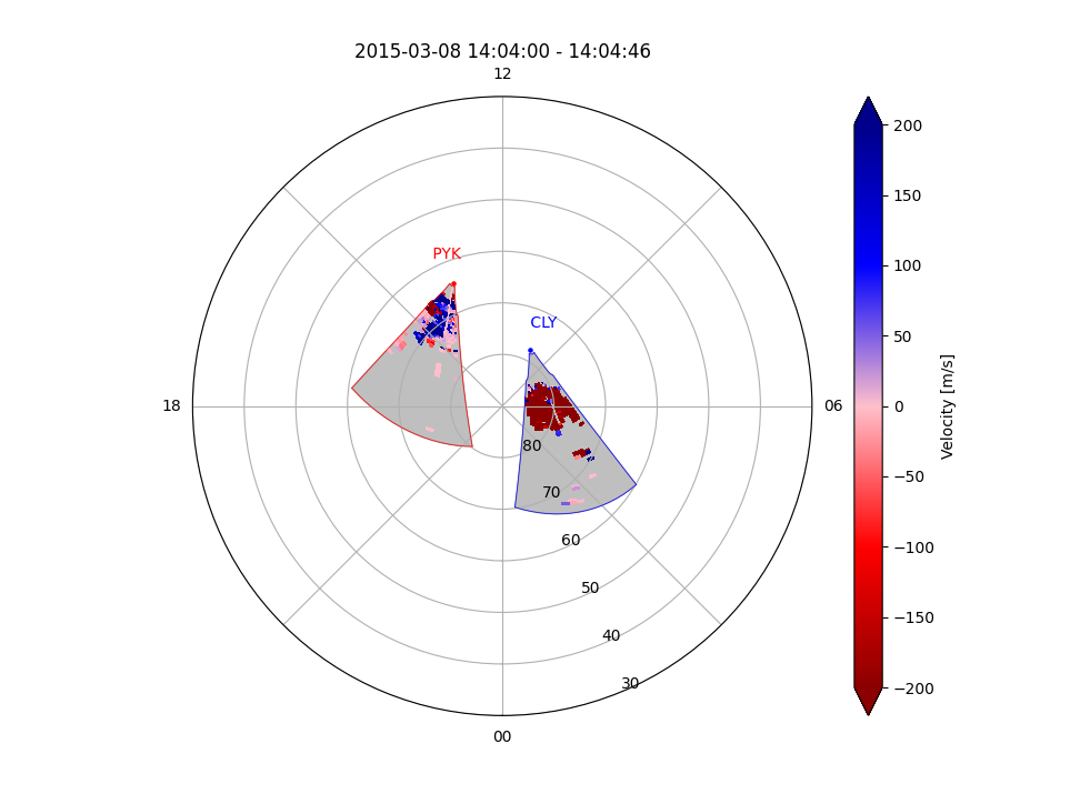
plot_fan can concatenate with itself, here is an example of plotting two different radars with some of the above parameters, remember to pass in the axes object (ax) to any subsequent plots, unlike the FOV plots, fan plots will automatically control the ccrs variable for you:

import pydarn
from datetime import datetime
import matplotlib.pyplot as plt 

cly_file = 'data/20150308.1400.03.cly.fitacf'
pyk_file = 'data/20150308.1401.00.pyk.fitacf'

pyk_data, _ = pydarn.read_dmap(pyk_file)
cly_data, _ = pydarn.read_dmap(cly_file)

fan_rtn = pydarn.Fan.plot_fan(cly_data, scan_time=datetime(2015, 3, 8, 14, 4),
                    colorbar=False, fov_color='grey', line_color='blue',
                    radar_label=True)

pydarn.Fan.plot_fan(pyk_data, scan_time=datetime(2015, 3, 8, 14, 4), 
                    colorbar_label='Velocity [m/s]', fov_color='grey',
                    line_color='red', radar_label=True, ax=fan_rtn['ax'])

plt.show()

Coastlines

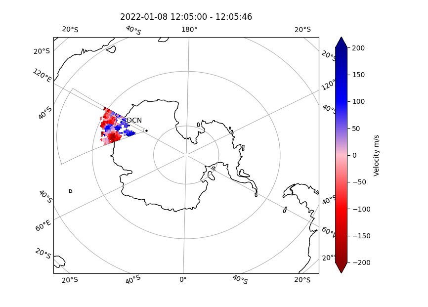
Plot an underlaid coastline map using the coastline keyword, this example also shows the use of plotting in geographic coordinates:

pydarn.Fan.plot_fan(data, scan_index=5, radar_label=True,
                    groundscatter=True,
                    coords=pydarn.Coords.GEOGRAPHIC,
                    projs=pydarn.Projs.GEO,
                    colorbar_label="Velocity m/s",
                    coastline=True)
plt.show()

User Input Data Fan Plots

As the scope of SuperDARN data expands, new control programs and modes of data collection are established, along with user requirements to average scans or plot non-standard data, it is increasingly difficult to develop an automatic fitacf to fan plot method that captures all of this nuance. In this case, we have introduced the user input fan plot where the user can make or massage data into their desired final product. As long as it fits into the fan plot array (e.g. 16 beams and 75 range gates) then the data can be plotted on a fan plot. This function also requires an identically sized array for groundscatter, if the user wishes. The following is an example of completely made up data, with some ground scatter and ranges without data:

import matplotlib.pyplot as plt
import pydarn
import datetime as dt
import numpy as np

# Test completely made up data for SAS
# Made up data in format [75, 16]
data_array = [(np.ones(16) * (x - 36) * 10).tolist() for x in range(75)]
# Add some areas with no data
for i in range(65,70):
    data_array[i] = (np.empty(16) * np.nan).tolist()

# Made up groundscatter boolean array
data_groundscatter = [(np.zeros(16)).tolist() for x in range(75)]
for i in range(30,40):
    data_groundscatter[i] = (np.ones(16)).tolist()

data_datetime = dt.datetime(2024,1,1,0,0)

pydarn.Fan.plot_fan_input(data_array=data_array,
                          data_datetime=data_datetime,
                          stid=pydarn.RadarID.SAS,
                          data_groundscatter = data_groundscatter,
                          data_parameter='v',
                          zmin=-400,zmax=400, lowlat=50, coastline=True)
plt.show()